pacman::p_load(jsonlite, tidygraph, ggraph,
               visNetwork, graphlayouts, ggforce,
               skimr, tidytext, tidyverse, ggplot2)

mc3_data <- fromJSON("data/MC3.json")1. Overview
Through visual analytics, FishEye aims to identify companies potentially engaged in illegal fishing and protect marine species affected by it.
In this context, this page will attempt to answer the following task under Mini-Challenge 3 of the VAST Challenge: Use visual analytics to identify anomalies in the business groups present in the knowledge graph. Limit your response to 400 words and 5 images.
1.1 Import Libraries and Datasets
The following code snippet will be utilized to install and import the required R packages for tasks related to data import, preparation, data manipulation, data analysis, and data visualization.
1.2 Extract Edges
The provided code snippet will extract the links data.frame from the mc3_data and store it as a tibble data.frame named mc3_edges.
Show the code
mc3_edges <- as_tibble(mc3_data$links) %>%
  distinct() %>%
  mutate(source = as.character(source),
         target = as.character(target),
         type = as.character(type)) %>%
  group_by(source, target, type) %>%
    summarise(weights = n()) %>%
  filter(source!=target) %>%
  ungroup()
1.3 Extract & View Nodes
The code snippet below will extract the nodes data.frame from mc3_data and store it as a tibble data.frame named mc3_nodes.
Show the code
mc3_nodes <- as_tibble(mc3_data$nodes) %>%
  mutate(country = as.character(country),
         id = as.character(id),
         product_services = as.character(product_services),
         revenue_omu = as.numeric(as.character(revenue_omu)),
         type = as.character(type)) %>%
  select(id, country, type, revenue_omu, product_services)

mc3_nodes
# A tibble: 27,622 × 5
id country type revenue_omu product_services
<chr> <chr> <chr> <dbl> <chr>
1 Jones LLC ZH Comp… 310612303. Automobiles
2 Coleman, Hall and Lopez ZH Comp… 162734684. Passenger cars,…
3 Aqua Advancements Sashimi SE Expr… Oceanus Comp… 115004667. Holding firm wh…
4 Makumba Ltd. Liability Co Utopor… Comp… 90986413. Car service, ca…
5 Taylor, Taylor and Farrell ZH Comp… 81466667. Fully electric …
6 Harmon, Edwards and Bates ZH Comp… 75070435. Discount superm…
7 Punjab s Marine conservation Riodel… Comp… 72167572. Beef, pork, chi…
8 Assam Limited Liability Company Utopor… Comp… 72162317. Power and Gas s…
9 Ianira Starfish Sagl Import Rio Is… Comp… 68832979. Light commercia…
10 Moran, Lewis and Jimenez ZH Comp… 65592906. Automobiles, tr…
# ℹ 27,612 more rows1.3.1 Check Missing value in Nodes
colSums(is.na(mc3_nodes)) id country type revenue_omu
0 0 0 21515
product_services
0 21515 missing from revenue_omu column
1.3.2 Check Duplicates in Nodes
mc3_nodes[duplicated(mc3_nodes),]# A tibble: 2,595 × 5
id country type revenue_omu product_services
<chr> <chr> <chr> <dbl> <chr>
1 Smith Ltd ZH Company NA Unknown
2 Williams LLC ZH Company NA Unknown
3 Garcia Inc ZH Company NA Unknown
4 Walker and Sons ZH Company NA Unknown
5 Walker and Sons ZH Company NA Unknown
6 Smith LLC ZH Company NA Unknown
7 Smith Ltd ZH Company NA Unknown
8 Romero Inc ZH Company NA Unknown
9 Niger River Marine life Oceanus Company NA Unknown
10 Coastal Crusaders AS Industrial Oceanus Company NA Unknown
# ℹ 2,585 more rows
Note
There are 2595 duplicates entries, which will be taken care of at a later part of code chunks
1.3.3 Remove dupliated rows in Nodes
mc3_nodes_unique <- distinct(mc3_nodes)

mc3_nodes_unique
# A tibble: 25,027 × 5
id country type revenue_omu product_services
<chr> <chr> <chr> <dbl> <chr>
1 Jones LLC ZH Comp… 310612303. Automobiles
2 Coleman, Hall and Lopez ZH Comp… 162734684. Passenger cars,…
3 Aqua Advancements Sashimi SE Expr… Oceanus Comp… 115004667. Holding firm wh…
4 Makumba Ltd. Liability Co Utopor… Comp… 90986413. Car service, ca…
5 Taylor, Taylor and Farrell ZH Comp… 81466667. Fully electric …
6 Harmon, Edwards and Bates ZH Comp… 75070435. Discount superm…
7 Punjab s Marine conservation Riodel… Comp… 72167572. Beef, pork, chi…
8 Assam Limited Liability Company Utopor… Comp… 72162317. Power and Gas s…
9 Ianira Starfish Sagl Import Rio Is… Comp… 68832979. Light commercia…
10 Moran, Lewis and Jimenez ZH Comp… 65592906. Automobiles, tr…
# ℹ 25,017 more rowsIn the following code chunk, the skim() function from the skimr package is employed to present the summary statistics of the mc3_edges tibble data frame.
1.4 Explore Edge data structure
skim(mc3_edges)| Name | mc3_edges |
| Number of rows | 24036 |
| Number of columns | 4 |
| _______________________ | |
| Column type frequency: | |
| character | 3 |
| numeric | 1 |
| ________________________ | |
| Group variables | None |
Variable type: character
| skim_variable | n_missing | complete_rate | min | max | empty | n_unique | whitespace |
|---|---|---|---|---|---|---|---|
| source | 0 | 1 | 6 | 700 | 0 | 12856 | 0 |
| target | 0 | 1 | 6 | 28 | 0 | 21265 | 0 |
| type | 0 | 1 | 16 | 16 | 0 | 2 | 0 |
Variable type: numeric
| skim_variable | n_missing | complete_rate | mean | sd | p0 | p25 | p50 | p75 | p100 | hist |
|---|---|---|---|---|---|---|---|---|---|---|
| weights | 0 | 1 | 1 | 0 | 1 | 1 | 1 | 1 | 1 | ▁▁▇▁▁ |
ggplot(data = mc3_edges,
       aes(x = type)) +
  geom_bar()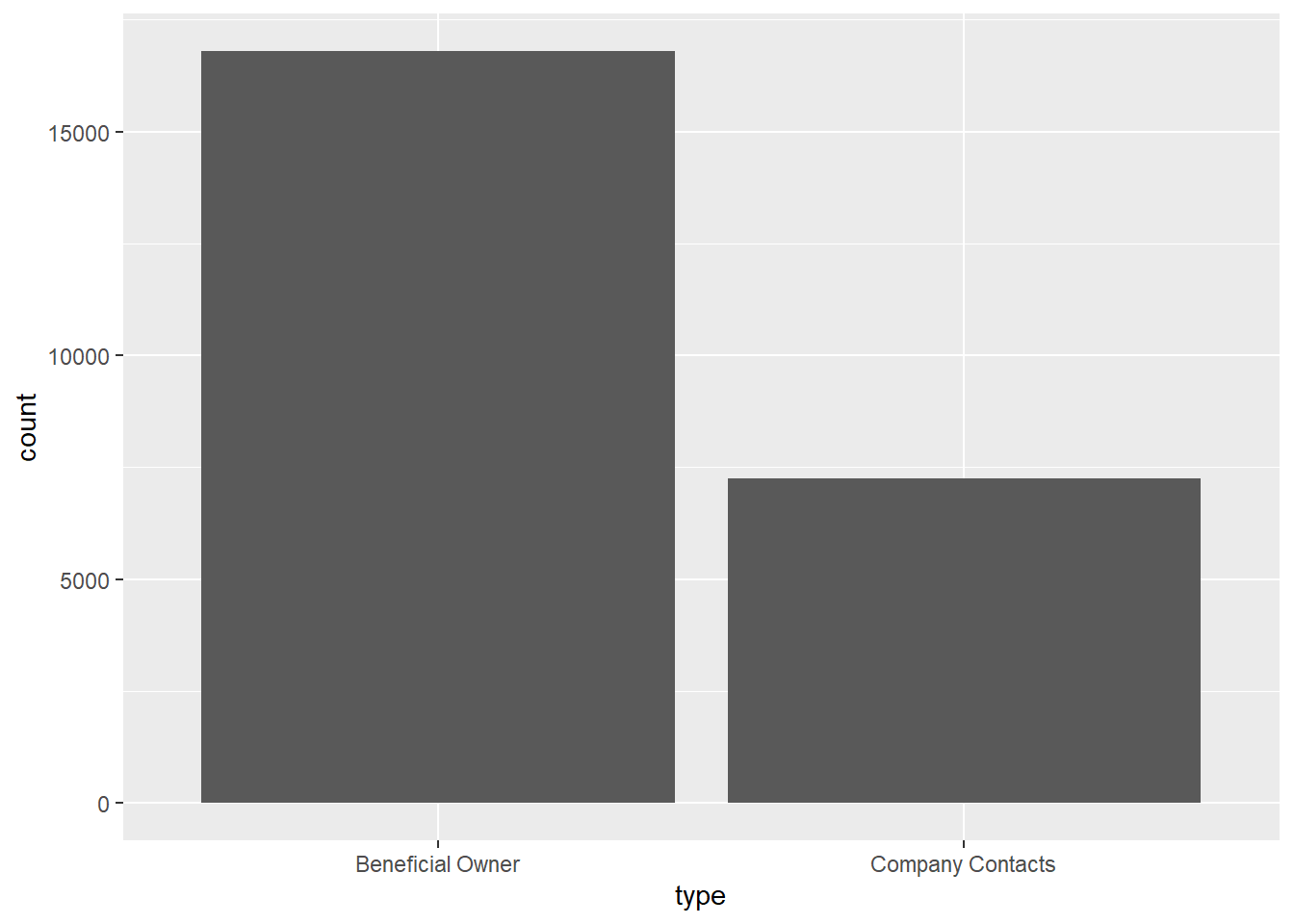
Note
We can also observe that there are Beneficial Owners than Company Contacts in terms of type.
1.5 Initial Network Graph Analysis
The following codes have been adapted largely from Professor Kam’s basic Network analysis Kick starter. It is noteworthy that the Prof filtered the data with those with betweenness centrality bigger than 100000.
id1 <- mc3_edges %>%
  select(source) %>%
  rename(id = source)
id2 <- mc3_edges %>%
  select(target) %>%
  rename(id = target)
mc3_nodes1 <- rbind(id1, id2) %>%
  distinct() %>%
  left_join(mc3_nodes,
            unmatched = "drop")

mc3_graph <- tbl_graph(nodes = mc3_nodes1,
                       edges = mc3_edges,
                       directed = FALSE) %>%
  mutate(betweenness_centrality = centrality_betweenness(),
         closeness_centrality = centrality_closeness())

mc3_graph %>%
  filter(betweenness_centrality >= 100000) %>%
ggraph(layout = "fr") +
  geom_edge_link(aes(alpha=0.5)) +
  geom_node_point(aes(
    linewidth = betweenness_centrality,
    colors = "lightblue",
    alpha = 0.5)) +
  scale_linewidth_continuous(range=c(1,10))+
  theme_graph() +
  theme(text = element_text(family = "sans"))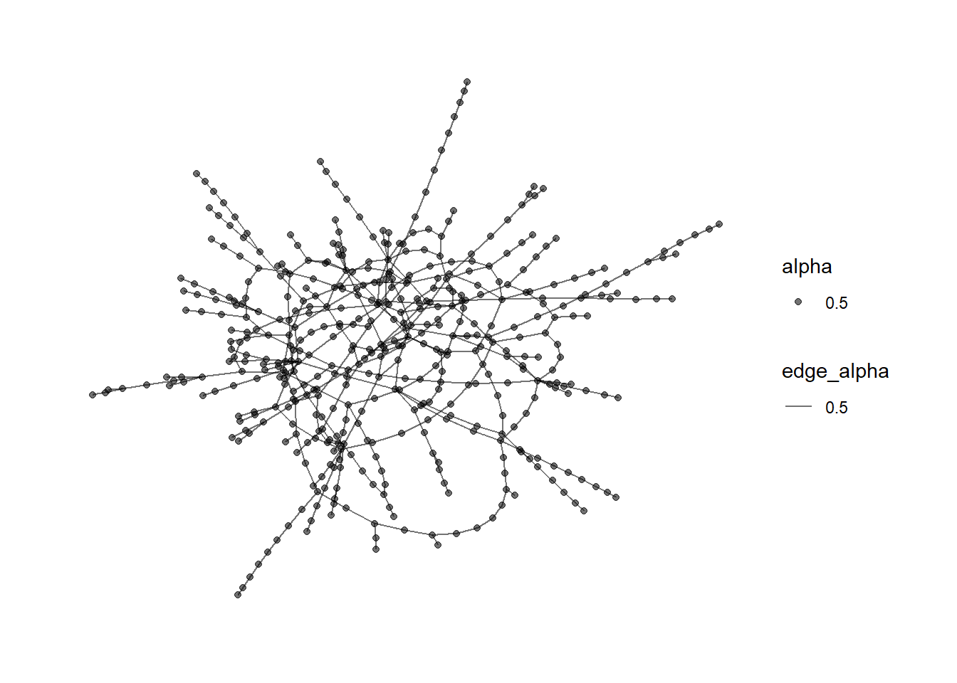
1.6 Explore Node data structure
The code below generates a table that displays the top 10 products or services based on their occurrence frequencies in the mc3_nodes_unique data frame.
top_products <- mc3_nodes_unique %>%
  count(product_services, sort = TRUE) %>%
  top_n(10)

# Rename the columns
top_products <- top_products %>%
  rename(Products = product_services, Occurrences = n)

# Print the table
print(top_products)
# A tibble: 10 × 2
Products Occurrences
<chr> <int>
1 character(0) 16395
2 Unknown 4614
3 Fish and seafood products 63
4 Seafood products 55
5 Fish and fish products 31
6 Food products 31
7 Canning, processing and manufacturing of seafood and other aquat… 23
8 Footwear 21
9 Seafood 20
10 Grocery products 19
Note
charactor(0) and Unknown will be cleaned later.
In the provided code chunk, the skim() function from the skimr package is utilized to present the summary statistics of the mc3_nodes tibble data frame. Also the distribution of Types. The result tells us there is no missing value in all fields, except revenue_omu.
skim(mc3_nodes)| Name | mc3_nodes |
| Number of rows | 27622 |
| Number of columns | 5 |
| _______________________ | |
| Column type frequency: | |
| character | 4 |
| numeric | 1 |
| ________________________ | |
| Group variables | None |
Variable type: character
| skim_variable | n_missing | complete_rate | min | max | empty | n_unique | whitespace |
|---|---|---|---|---|---|---|---|
| id | 0 | 1 | 6 | 64 | 0 | 22929 | 0 |
| country | 0 | 1 | 2 | 15 | 0 | 100 | 0 |
| type | 0 | 1 | 7 | 16 | 0 | 3 | 0 |
| product_services | 0 | 1 | 4 | 1737 | 0 | 3244 | 0 |
Variable type: numeric
| skim_variable | n_missing | complete_rate | mean | sd | p0 | p25 | p50 | p75 | p100 | hist |
|---|---|---|---|---|---|---|---|---|---|---|
| revenue_omu | 21515 | 0.22 | 1822155 | 18184433 | 3652.23 | 7676.36 | 16210.68 | 48327.66 | 310612303 | ▇▁▁▁▁ |
ggplot(data = mc3_nodes,
       aes(x = type)) +
  geom_bar()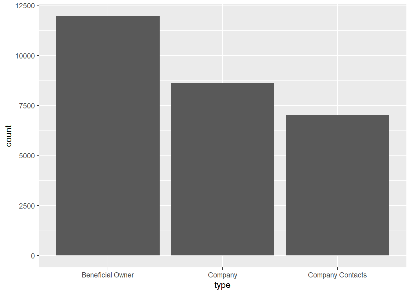
2 Text Analytics with tidytext
In this section, I will perform basic text sensing using appropriate functions of tidytext package.
2.1 Record those “Unknown” or”Charactor(0)” to “NA”
mc3_nodes$product_services[mc3_nodes$product_services == "Unknown"] <- NA
mc3_nodes$product_services[mc3_nodes$product_services == "character(0)"] <- NA
2.2 Tokenisation
token_nodes <- mc3_nodes %>%
  unnest_tokens(word,
                product_services,
                to_lower = TRUE,
    # Exclude punctuation from tokenisation result
                strip_punct = TRUE)
2.3 Visualize the words extracted
The below code generates a column plot that displays the count of the top 15 unique words found in the product_services field of the token_nodes data frame. The plot provides a visual representation of the word frequencies in the data. As you can see there are stopwords like “and”, “of”, “as”, and large number of “NA” which need to be cleaned up.
token_nodes %>%
  count(word, sort = TRUE) %>%
  top_n(15) %>%
  mutate(word = reorder(word, n)) %>%
  ggplot(aes(x = word, y = n)) +
  geom_col() +
  xlab(NULL) +
  coord_flip() +
      labs(x = "Count",
      y = "Unique words",
      title = "Count of unique words found in product_services field")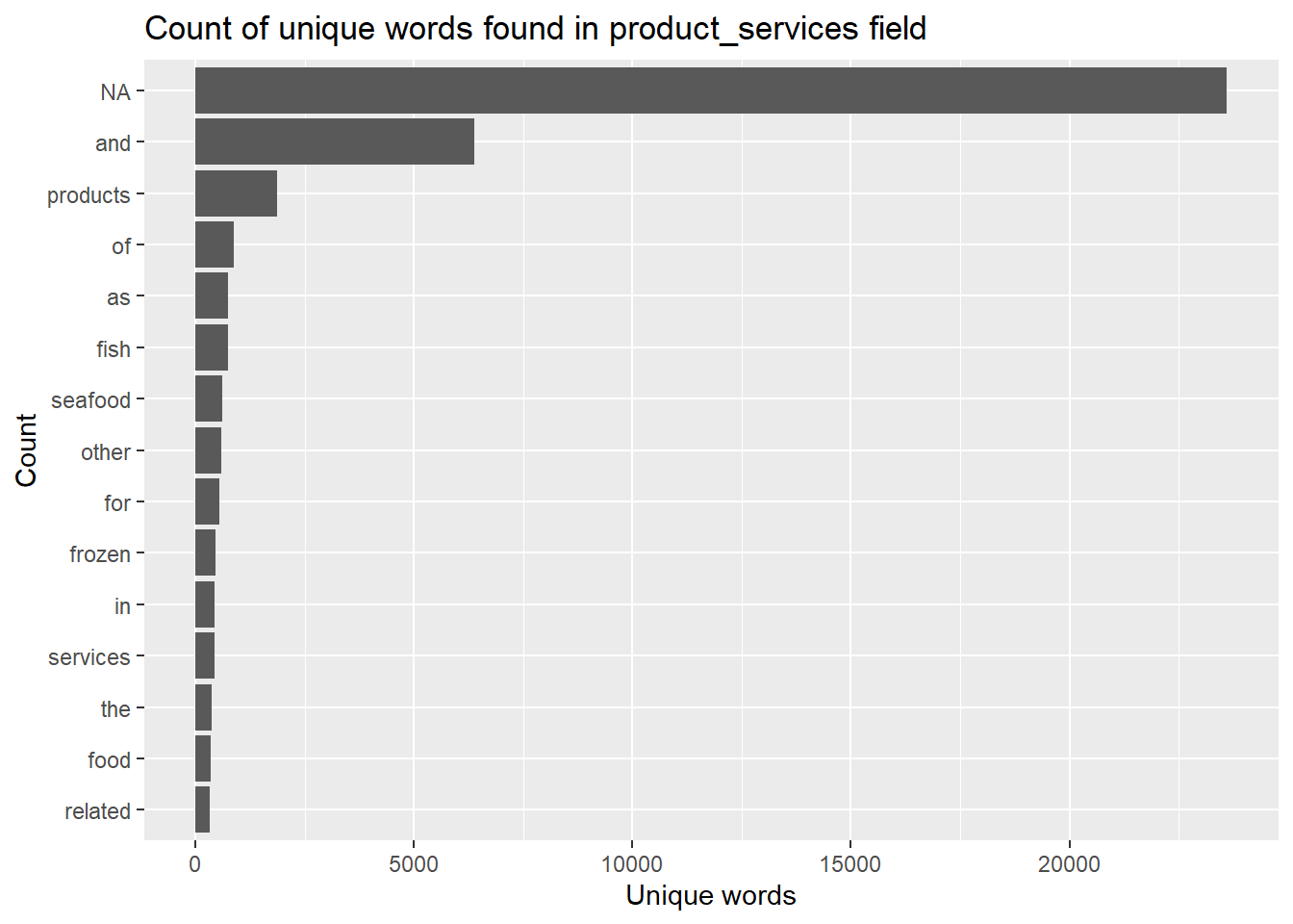
2.4 Remove the rows with stopwords and “NA”
stopwords_removed <- token_nodes %>%
  anti_join(stop_words)

stopwords_removed <- token_nodes %>%
  anti_join(stop_words) %>%
  filter(!is.na(word))

stopwords_removed %>%
  count(word, sort = TRUE) %>%
  top_n(15) %>%
  mutate(word = reorder(word, n)) %>%
  ggplot(aes(x = word, y = n)) +
  geom_col() +
  xlab(NULL) +
  geom_text(aes(label = n), vjust = 0.5, hjust = -0.1, size = 2, color = "black")+
  coord_flip() +
      labs(x = "Count",
      y = "Unique words",
      title = "Count of Top 15 unique words found in product_services field")+
theme_minimal() 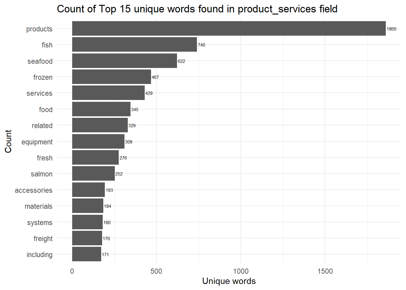
2.4.1 Count of words after removing stopwords and NA
We will compare the count of words before and after the clean up.
stopwords_removed_unique <- stopwords_removed %>%
  filter(!is.na(word))

print("length before stopwords removal")
[1] "length before stopwords removal"length(unique(stopwords_removed_unique$word))[1] 7747print("length after stopwords removal")[1] "length after stopwords removal"length(unique(token_nodes$word))[1] 8034
Note
About ~200 unique words have been removed as part of stopwords removal. However, there are still with a lot of words not related to fishery
2.6 Match ID from Nodes to Source in Edge
The below code filters and extracts specific rows from the mc3_edges and mc3_nodes_fishery data frames based on certain conditions and stores the filtered data in new variables (mc3_edges_new and mc3_nodes_fishery_new). The operations are performed to retain only the relevant edges and nodes related to the selected targets and remove the unnecessary ones (Non_targets).
Show the code
targets <- mc3_edges %>%
  filter(source %in% mc3_nodes_fishery$id) %>%
  select(target)

#Filter mc_edges with  the extracted targets
mc3_edges_new <- mc3_edges %>%
  filter(target %in% targets$target)

#Define "Non_targets" a targets that are not selected from mc3_edges

Non_targets <- mc3_edges %>%
  filter(!target %in% targets$target) %>%
  distinct(target, .keep_all = TRUE)

#Remove non_targets from Node_fishery
mc3_nodes_fishery_new <- mc3_nodes_fishery %>%
  filter(!mc3_nodes_fishery$id %in% Non_targets$source)
2.8 Additional Data Clean Ups
Based on a quick skim below, the maximum length of Source in the edges data is whopping 213, this is likely an input with lot of c(“,”) values.
skim(mc3_edges_new)| Name | mc3_edges_new |
| Number of rows | 3711 |
| Number of columns | 4 |
| _______________________ | |
| Column type frequency: | |
| character | 3 |
| numeric | 1 |
| ________________________ | |
| Group variables | None |
Variable type: character
| skim_variable | n_missing | complete_rate | min | max | empty | n_unique | whitespace |
|---|---|---|---|---|---|---|---|
| source | 0 | 1 | 7 | 213 | 0 | 1493 | 0 |
| target | 0 | 1 | 6 | 27 | 0 | 2887 | 0 |
| type | 0 | 1 | 16 | 16 | 0 | 2 | 0 |
Variable type: numeric
| skim_variable | n_missing | complete_rate | mean | sd | p0 | p25 | p50 | p75 | p100 | hist |
|---|---|---|---|---|---|---|---|---|---|---|
| weights | 0 | 1 | 1 | 0 | 1 | 1 | 1 | 1 | 1 | ▁▁▇▁▁ |
2.8.1 Clean up Source Values
mc3_edges_new_filtered <- mc3_edges_new %>%
  filter(startsWith(source, "c("))

#step 2

mc3_edges_new_split <- mc3_edges_new_filtered %>%
  separate_rows(source, sep = ", ") %>%
  mutate(source = gsub('^c\\(|"|\\)$', '', source))

#remove rows with grouped

mc3_edges_new2 <- mc3_edges_new %>%
  anti_join(mc3_edges_new_filtered)

#Add rows in step #2

mc3_edges_new2 <- mc3_edges_new2 %>%
  bind_rows(mc3_edges_new, mc3_edges_new_split)

#group

mc3_edges_new_groupby <- mc3_edges_new2 %>%
  group_by(source, target, type) %>%
  summarize(weight = n()) %>%
  filter(weight >1) %>%
  ungroup()
From another skim below, the maximum length of source has reduced from 213 to 57, after removing lot of c(“,”) values.
skim(mc3_edges_new_groupby)| Name | mc3_edges_new_groupby |
| Number of rows | 3703 |
| Number of columns | 4 |
| _______________________ | |
| Column type frequency: | |
| character | 3 |
| numeric | 1 |
| ________________________ | |
| Group variables | None |
Variable type: character
| skim_variable | n_missing | complete_rate | min | max | empty | n_unique | whitespace |
|---|---|---|---|---|---|---|---|
| source | 0 | 1 | 7 | 57 | 0 | 1485 | 0 |
| target | 0 | 1 | 6 | 27 | 0 | 2887 | 0 |
| type | 0 | 1 | 16 | 16 | 0 | 2 | 0 |
Variable type: numeric
| skim_variable | n_missing | complete_rate | mean | sd | p0 | p25 | p50 | p75 | p100 | hist |
|---|---|---|---|---|---|---|---|---|---|---|
| weight | 0 | 1 | 2 | 0.09 | 2 | 2 | 2 | 2 | 5 | ▇▁▁▁▁ |
class(mc3_edges_new_groupby)[1] "tbl_df" "tbl" "data.frame"2.9 Link the latest edges to the nodes
The code below performs data manipulation and transformation tasks to handle missing or incomplete data in the mc3_nodes_fishery_new data frame. It creates rows for sources and targets, combines them with the filtered nodes data, and summarizes the information by grouping it based on the id column.
source_missing <-setdiff(mc3_edges_new_groupby$source, mc3_nodes_fishery_new$id)

source_missing_df <- tibble(
  id = source_missing,
  country = rep(NA_character_, length(source_missing)),
  type = rep("Company", length(source_missing)),
  revenue = rep(NA_real_, length(source_missing)),
  product_services = rep(NA_character_, length(source_missing))
)

target_missing <- setdiff(mc3_edges_new_groupby$target, mc3_nodes_fishery_new$id)

target_missing_df <- tibble(
  id = target_missing,
  country = rep(NA_character_, length(target_missing)),
  type = rep("Company", length(target_missing)),
  revenue = rep(NA_real_, length(target_missing)),
  product_services = rep(NA_character_, length(target_missing))
)

#Keep only id values from Nodes df also present in the edges df
mc3_nodes_fishery_new_filtered <- mc3_nodes_fishery_new %>%
  filter(id %in% c(mc3_edges_new_groupby$source, mc3_edges_new_groupby$target))

mc3_nodes_fishery_new_df <- bind_rows(mc3_nodes_fishery_new_filtered, source_missing_df, target_missing_df)

mc3_nodes_fishery_new_df <- mc3_nodes_fishery_new_df %>%
  mutate(revenue_omu = as.character(revenue_omu))

#Cleaned Nodes Dataframe grouped by Id
mc3_nodes_fishery_grouped <- mc3_nodes_fishery_new_df %>%
  group_by(id) %>%
  summarize(
    count = n(),
    type_1 = ifelse(n() >= 1, type[1], NA),
    type_2 = ifelse(n() >= 2, type[2], NA),
    type_3 = ifelse(n() >= 3, type[3], NA),
    country = ifelse(n() == 1, country, paste(unique(country), collapse = ", ")),
    revenue_omu = ifelse(n() == 1, revenue_omu, paste(unique(revenue_omu), collapse = ", ")),
    product_services = ifelse(n() == 1, product_services, paste(unique(product_services), collapse = ", "))
  )

mc3_nodes_fishery_grouped
# A tibble: 4,372 × 8
id count type_1 type_2 type_3 country revenue_omu product_services
<chr> <int> <chr> <chr> <chr> <chr> <chr> <chr>
1 2 Limited Li… 1 Compa… <NA> <NA> Marebak <NA> Canning, proces…
2 3 Ltd. Liabi… 1 Compa… <NA> <NA> Oceanus 112666.6728 European specia…
3 7 Ltd. Liabi… 1 Compa… <NA> <NA> <NA> <NA> <NA>
4 8 SE Marine … 1 Compa… <NA> <NA> <NA> <NA> <NA>
5 9 Charter Bo… 1 Compa… <NA> <NA> Marebak 36658.0122 Fish and fish p…
6 9 Shark S.A.… 1 Compa… <NA> <NA> <NA> <NA> <NA>
7 9 Swordfish … 1 Compa… <NA> <NA> <NA> <NA> <NA>
8 Aaron Carr 1 Compa… <NA> <NA> <NA> <NA> <NA>
9 Aaron Donald… 1 Compa… <NA> <NA> <NA> <NA> <NA>
10 Aaron Lee 1 Compa… <NA> <NA> <NA> <NA> <NA>
# ℹ 4,362 more rows3 Network Analysis with Refined Graph with the Fishery edges and nodes
mc3_fish_graph <- tbl_graph(nodes = mc3_nodes_fishery_,
                       edges = mc3_edges_fishery,
                       directed = FALSE) %>%
  mutate(betweenness_centrality = centrality_betweenness()) %>%
  filter(betweenness_centrality >= 10000) %>%
  ggraph(layout = "nicely") +
  scale_edge_width(range = c(0.01, 6)) +
  geom_node_point(aes(colour = type_1,
                      size = betweenness_centrality)) +
  theme_graph() +
  labs(size = "Betweenness Centrality")

mc3_fish_graph 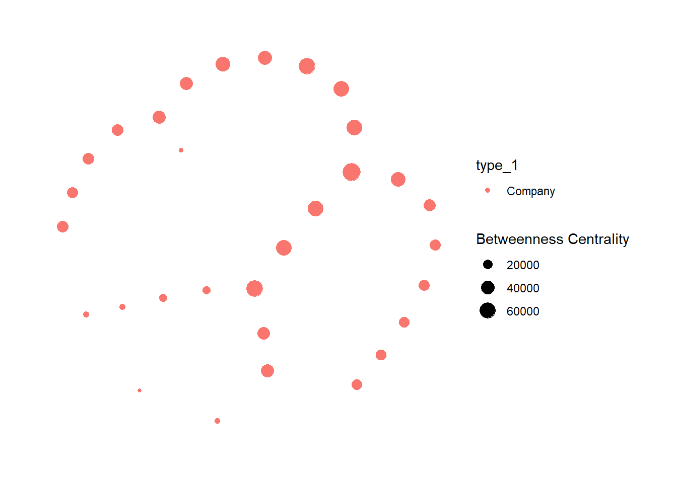
Note
I can observe that all of the refined Nodes with betweeness centrality greater than 10,000 has type equal to “Company”, with a few nodes with relatively high betweenness centrality near to the center
3.1 Find Targets () linked to multiple companies, which may be indications of anomalies.
mc3_edges_fishery %>%
  group_by(target) %>%
  filter(n_distinct(source) > 1) %>%
  select(target)
# A tibble: 1,324 × 1
# Groups: target [508]
target
<chr>
1 Elizabeth Jones
2 Michael Morrison
3 Amanda Robinson
4 Andrew Taylor
5 Brandon Cruz
6 Michael Thompson
7 Melissa Martin
8 Christopher Ramos
9 Richard Smith
10 Andrew Reed
# ℹ 1,314 more rowsmc3_edges_fishery %>%
group_by(target) %>%
summarise(count = n()) %>%
arrange(desc(count)) %>%
select(target, count)# A tibble: 2,887 × 2
target count
<chr> <int>
1 Michael Johnson 11
2 John Smith 10
3 Brian Smith 8
4 Jennifer Johnson 8
5 Michael Smith 8
6 Richard Smith 8
7 David Smith 7
8 James Brown 7
9 James Smith 7
10 Melissa Brown 7
# ℹ 2,877 more rowsmc3_edges_fishery_in <- mc3_edges_fishery %>%
rename(from = source, to = target)
mc3_nodes_fishery_in <- mc3_nodes_fishery_ %>%
rename(group = type_1) 3.2 Distribution of Targets linked to multiple companies
filtered_data <- mc3_edges_fishery %>%
  group_by(target) %>%
  summarise(count = n()) %>%
  arrange(desc(count)) %>%
  select(target, count)

filtered_data %>%
  group_by(count) %>%
  summarise(n = n()) %>%
  mutate(percentage = round(n/sum(n) * 100, 2)) %>%
  ggplot(aes(x = count, y = n, label = paste0(round(percentage, 2), "%"))) +
  geom_bar(stat = "identity", fill = "lightblue", color = "black") +
  xlab("Number of Ownership") +
  ylab("Count") +
  scale_x_continuous(breaks = unique(filtered_data$count)) +
  geom_text(position = position_dodge(width = 0.9), vjust = -0.5, size = 4) +
  ggtitle("Distribution of the Number of Ownership") +
  theme_minimal() +
  labs(
    x = "Number of Ownership",
    y = "Count",
    fill = "Number of Ownership"
  )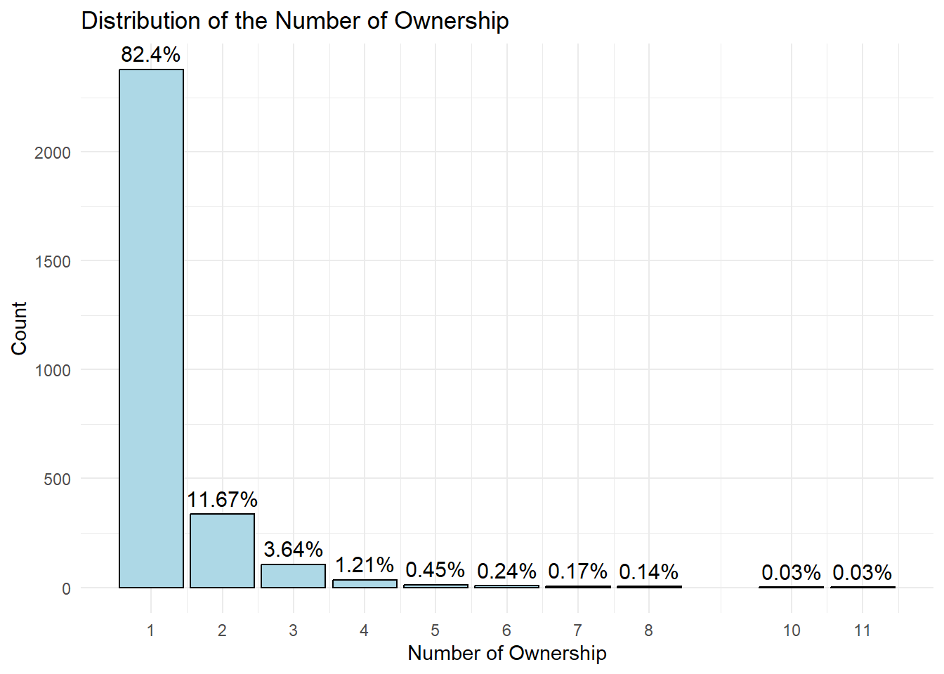
Note
Nearly 80% of the targets have count of 1. I have decided to use the Pareto rules to look at the top 20% only.
3.2.1 Distribution of Targets linked to at least 2 companies
filtered_data2 <- mc3_edges_fishery %>%
  group_by(target) %>%
  summarise(count = n()) %>%
  filter(count > 1) %>%
  arrange(desc(count)) %>%
  select(target, count)

filtered_data2 %>%
  group_by(count) %>%
  summarise(n = n()) %>%
  mutate(percentage = round(n/sum(n) * 100, 2)) %>%
  ggplot(aes(x = count, y = n, label = paste0(round(percentage, 2), "%"))) +
  geom_bar(stat = "identity", fill = "lightblue", color = "black") +
  xlab("Number of Ownership") +
  ylab("Count") +
  scale_x_continuous(breaks = unique(filtered_data$count)) +
  geom_text(position = position_dodge(width = 0.9), vjust = -0.5, size = 4) +
  ggtitle("Distribution of the Number of Ownership") +
  theme_minimal() +
  labs(
    x = "Number of Ownership",
    y = "Count",
    fill = "Number of Ownership"
  )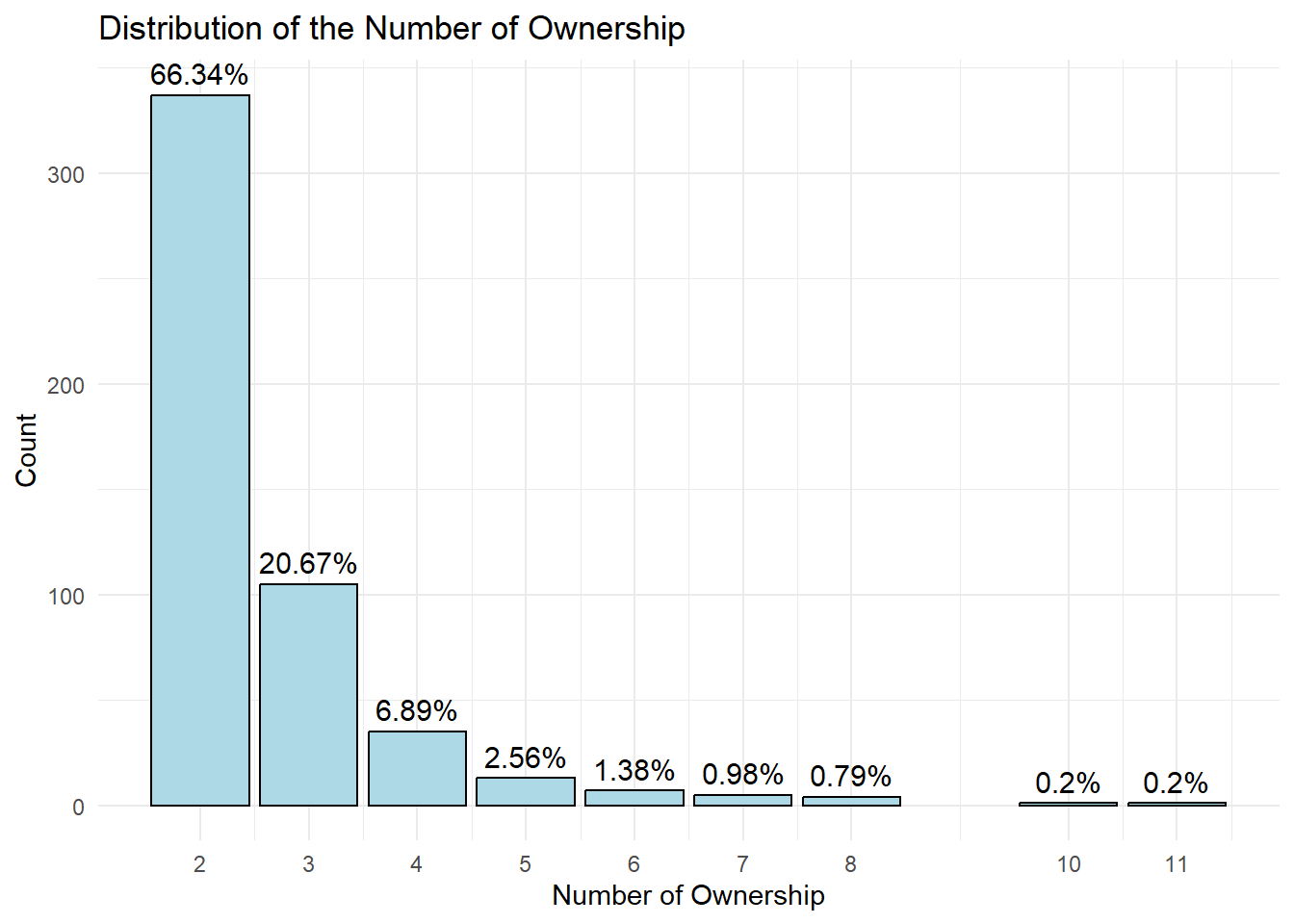
Note
We are now left with about 500 companies. The future work is that there should be a way to define a cut-off value on company ownership for creating a subgraph that focuses on company owners who own relatively higher number of comapnies. Conscious of time, I have decided to look at just top 5 targets in terms of the number of counts, starting with Michael Johnson, who has the highest number of counts.
3.2.2 Network Analysis on Michael Johnson
Michael_Johnson <- unique(mc3_edges_fishery_in$from[mc3_edges_fishery_in$to == "Michael Johnson"])
Michael_Johnson_edges <- subset(mc3_edges_fishery_in, from %in% Michael_Johnson)
Michael_Johnson_nodes <- subset(mc3_nodes_fishery_, id %in% c(Michael_Johnson_edges$from, Michael_Johnson_edges$to))

# Create a visNetwork
visNetwork(nodes = Michael_Johnson_nodes, edges = Michael_Johnson_edges) %>%
  visIgraphLayout(layout = "layout_with_fr") %>%
  visOptions(highlightNearest = TRUE, nodesIdSelection = TRUE) %>%
  visLegend() %>%
  visLayout(randomSeed = 123)
Note
Michael Johnson is a sole owner of many smaller entities. Revenue of most of the companies are unknown, hinting to us that some of these might be paper companies
3.2.3 Network Analysis on Top 5 Targets
top5 <- mc3_edges_fishery_in$from[mc3_edges_fishery_in$to %in% c("Michael Johnson", "John Smith", "Brian Smith", "Jennifer Johnson", "Michael Smith")]

top5_edges <- subset(mc3_edges_fishery_in, from %in% top5)

top5_nodes <- subset(mc3_nodes_fishery_, id %in% c(top5_edges$from, top5_edges$to))


# Create a visNetwork
visNetwork(nodes = top5_nodes, edges = top5_edges) %>%
  visIgraphLayout(layout = "layout_with_fr") %>%
  visOptions(highlightNearest = TRUE, nodesIdSelection = TRUE) %>%
  visLegend() %>%
  visLayout(randomSeed = 123)
Note
The analysis on Top 5 targets verifies that Michael Johnson is not a unique case. Top 5 targets are sole owners of many smaller entities. Revenue of most of the companies they own are also unknown, hinting to us some of these might be paper companies possibly involved in transshipment.
4 Conclusion
Through data exploration, I was able to observe a few anomalies.
Individuals who have ownership in multiple companies. From analyzing three sub-network graphs, it was observed that these individuals tend to own a combination of large and small firms from various countries. While there is a possibility that everything is legitimate, it would be beneficial for FishEye to conduct a thorough examination of these individuals who own companies across borders, particularly when they are the sole owners of smaller entities, as exemplified in the case of ‘Michael Johnson’ and other top targets. Revenue of most of the companies they own are unknown from the data given, which may require authorities and authorities’ scrutiny.
Almost all of the refined Nodes has type equal to “Company”, there were no beneficial owners and company contacts. This is expected looking from the distribution of types for Node Dataframe intiially, but it would be noteworthy for authorities to investigate further if this conceration of one id type has linkages with illegal fishery.